SPECIES DIVERSITY

Popular estimates of biodiversity value:
using species richness

Species richness
Comparing 'indicator' groups

Fortunately, when dealing with large numbers of species, species richness tends to become a reasonable surrogate for gene or character richness (ref 4). Therefore identifying genes or characters as a fundamental currency of biodiversity value provides an additional justification for using species richness. This is likely to work because (unlike the bumble bee example) as more species are added in total, at least some representatives of the more divergent, higher groups of organisms (which taken together are rich in different characters) usually co-occur.

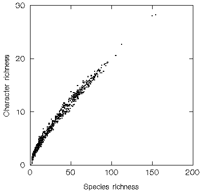
This relationship may be illustrated by joint work with the Royal Botanic Gardens, Kew, which examined species richness for five plant families (Dichapetalaceae, Lecythidaceae, Caryocaraceae, Chrysobalanaceae and Proteaceae genus Panopsis) from the long-running Flora Neotropica project among one-degree grid cells (ref 5). The five families include 729 species, and the best available estimate of character richness had to be derived from the current taxonomic classification. Although this is likely to underestimate the degree of character divergence between some species, this is the same method that is used for the bumble bee example in the description of estimates of genetic or character richness, and yet the relationship between species richness and character richness for this much larger group is much closer (below):

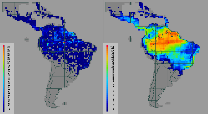
However, using species richness as a surrogate for gene or character richness is still not a panacea, because there are probably too many species even within a suburban garden for complete enumeration, let alone for surveys extending across large regions, such as South America. The problems are illustrated by the same Flora Neotropica data. The five families include 729 species among 1751 grid cells, thereby requiring over one million presence/absence records to be established. Such an enormous sampling effort cannot be deployed quickly and is very expensive. The example shows relative counts of the numbers of species from these five plant families (before, left, and after, right, interpolating the sample data to model the expected distributions of species), with the richer areas shown in orange and the poorer areas shown in dark blue (the score classes on the left are arranged in equal richness intervals, whereas on the right they are arranged for equal numbers of grid cells) (ref 5) (below):

specimen records interpolated records

Comparing 'indicator groups'

The use of surrogates, in the broadest sense, may be applied to address two problems: first, just as in the Flora Neotropica example for five families of trees above, how good is the species richness of tree floras at predicting the character richness of tree floras?; and second, how good is it for predicting the species and character richness of other groups, or of entire biotas, as an 'indicator group'? The latter, inter-group relationship can be predictive under some circumstances. However, indicator relationships cannot always be assumed, because they can also be weak, absent or even negative, perhaps particularly when indicator and target organisms differ in their habitat associations because different factors govern their distributions.

The geographical patterns of diversity for two groups of organisms can be compared graphically by overlaying the two maps in two separate colours (ref 14). Here, increasing intensity of green is used to represent increasing species richness of butterflies in the first map (data used with permission of the Biological Records Centre), and increasing intensity of blue is used for species richness of birds in the second map (data used with permission of the British Trust for Ornithology). These green and blue maps are then overlaid in the third map. Consequently, black grid cells on the third map show low richness for both butterflies and birds; white shows high richness for both; and shades of grey show intermediate and covarying richness for both (these covarying scores lie on the diagonal of the colour key, to the left of the third map). In contrast, areas of the third map with highly saturated green cells show an excess of richness for butterflies over birds, and areas with highly saturated blue show an excess of birds over butterflies (Spearman correlation coefficient rho= 0.25). The colour classes are arranged to give even frequency distributions of richness scores along both axes (at least within the constraints imposed by tied richness scores) (below):

(201 Kb image)

Link to image building up overlays of butterflies and birds.

This technique allows relationships between groups to be compared visually at a broad range of spatial scales. Within Britain, for example, any gross differences in the strength of the overall national relationship can be judged from the overall colour saturation of the map; second, any regional deviations from this national relationship can be seen in regional colour trends; and third, local deviations can be seen as isolated spots of differing colour. The next example shows three overlay plots for all comparisons between birds and two insect groups, butterflies and dragonflies, as discussed in ref 14 (below):

(191 Kb image)

Link to images showing overlay comparison of birds, butterflies and dragonflies.

More strongly divergent patterns between some groups have long been known to natural historians. To take an example of European trees, using data from joint work with Raino Lampinen, Tapani Lahti and Pertti Uotila of the Atlas Florae Europaeae, there is a negative correlation between the distribution of species and subspecies richness of Pinaceae (pines, firs, spruces, larches) and the richness of Fagaceae (oaks, beeches and chestnut) (Spearman correlation coefficient rho= -0.33). Here, increasing intensity of blue is used to represent increasing native species and subspecies richness of Pinaceae and intensity of green is used for native species and subspecies richness of Fagaceae. In this case an indicator relationship would not be expected, because the two groups tend to have preferences for different climates. Many of the Pinaceae are a dominant component of the Boreal forests of northern and eastern Europe (blue), whereas the Fagaceae are a major component of the Southern-temperate forests of southern and western Europe (green). Nonetheless, in central Europe many species of the two groups occur in close proximity in the mountains (white or red: for example, on the southern side of the Alps), although often at different altitudes (below):

(103 Kb image)

Link to images showing overlay comparison of Pinaceae and Fagaceae.